Overview of Nonparametric Statistics
2/7/16
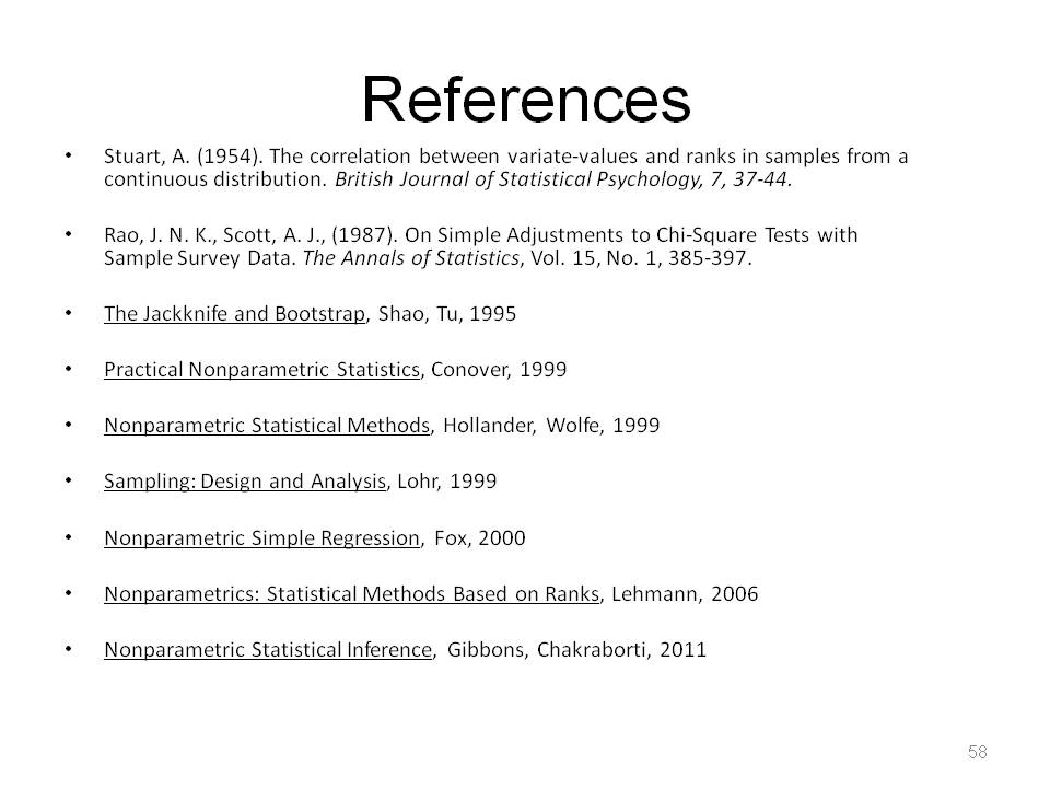
This is a slightly modified web version of a presentation I gave at work on nonparametric statistics and their use in survey work. I include all slides below, some notes for some slides, as well as a link to the .pdf file of the slides here. If you are interested in nonparametric statistics, I very strongly recommend checking out these books:
Nonparametric Statistical Methods by Hollander, Wolfe, and Chicken (lays out assumptions really well, has some theory), Nonparametrics: Statistical Methods Based on Ranks, by Lehmann, and Nonparametric Statistical Inference, by Gibbons and Chakraborti (has detailed theory at graduate level).
We use nonparametric statistics in survey work because we all start out doing design based sampling.
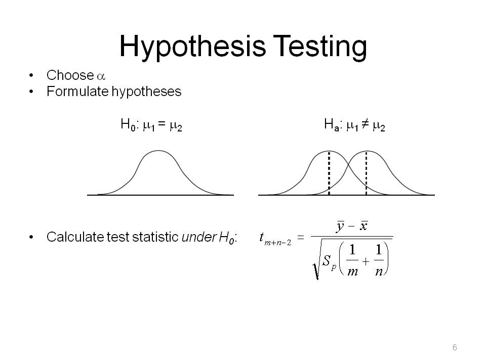
To talk about nonparametric statistics, you have to understand parametric statistics. We make assumptions about sampling distribution and test statistic (z-test, t-test, f-test).
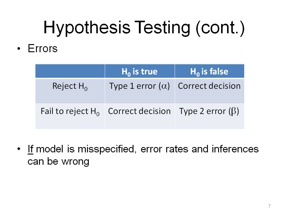
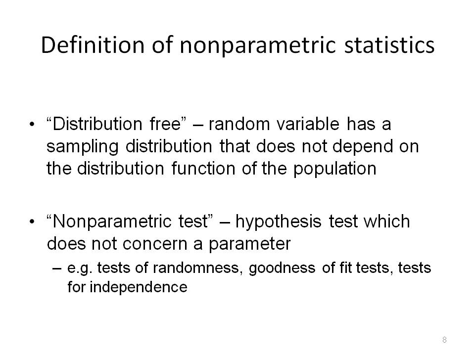
The term distribution free is a bit misleading. These are based on data characteristics such as order/rank, sign, or frequency and provide different ways of solving parametric problems. Nonparametric tests are not about parameters, so there is no counterpart in parametric statistics. These provide ways to verify assumptions of parametric statistics (e.g., randomness, normality).
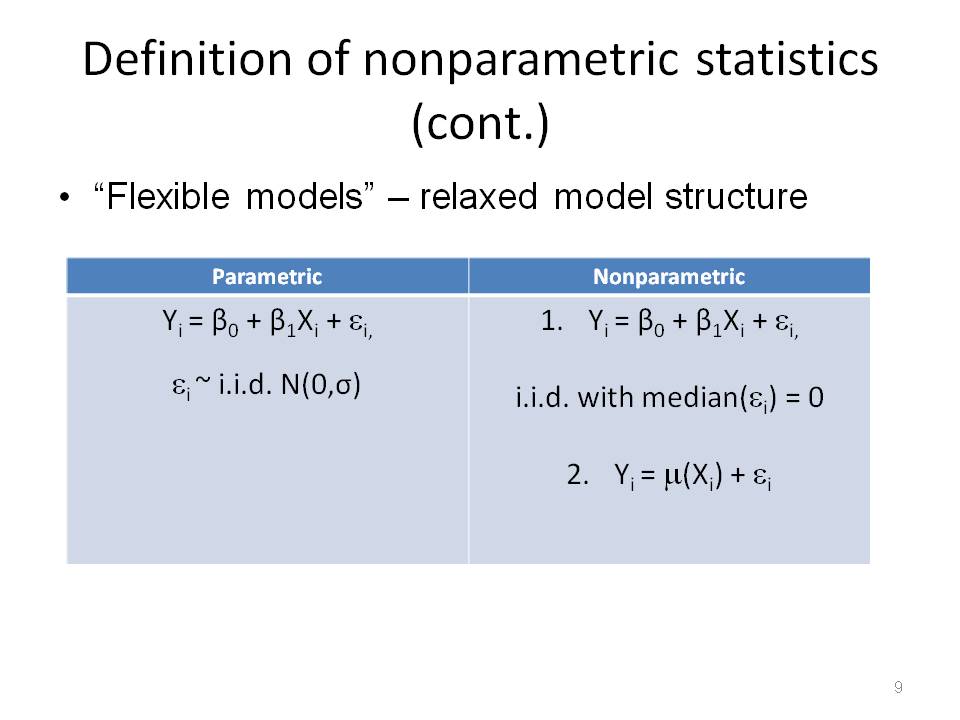
A few nonparametric regression options are to keep linear structure, but relax distribution assumptions on e's, or not keep linear structure at all, mu() is say a local average.
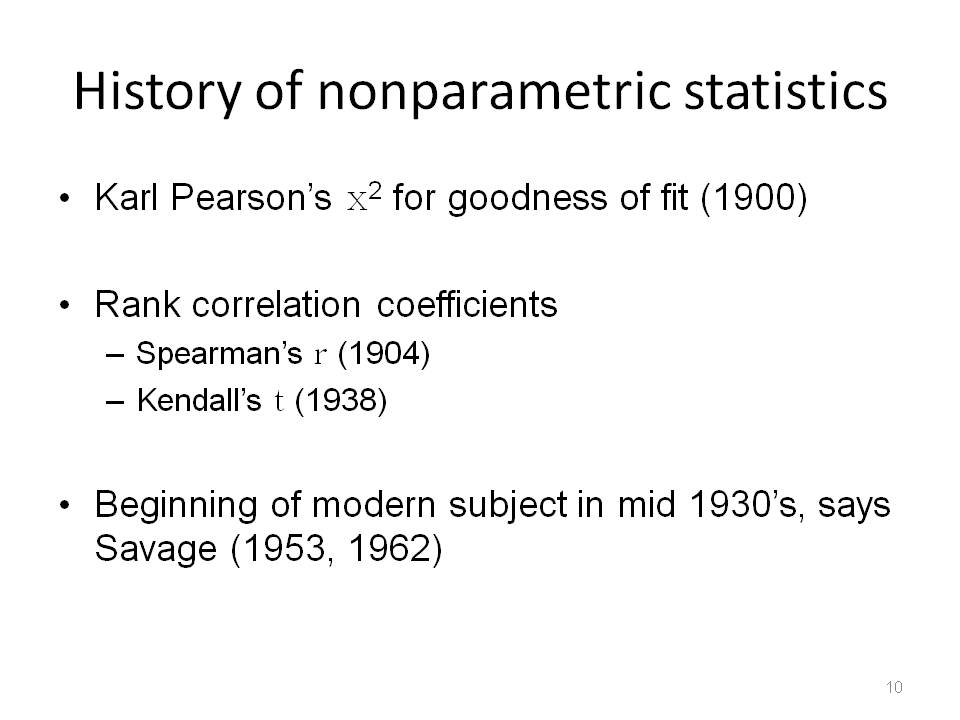
Here I pick and choose from about 100 years of history. We are familiar with the Pearson correlation coefficient. These correlation coefficients are nonparametric alternatives. Note that one cannot use a weight statement for Kendall's tau in SAS's PROC CORR.
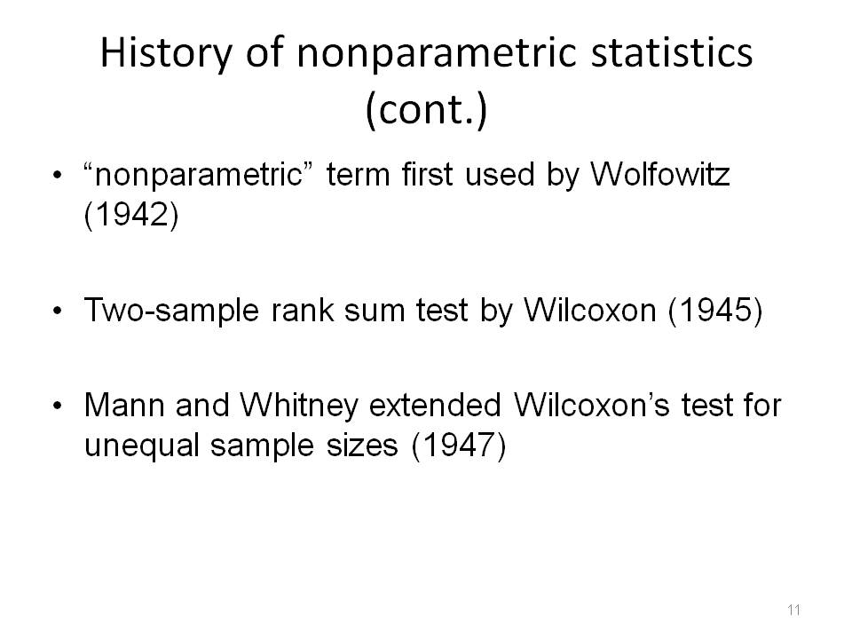
Wilcoxon (1945), started full-scale development of rank based methods. I will show an example of the Wilcoxon rank sum test in detail.
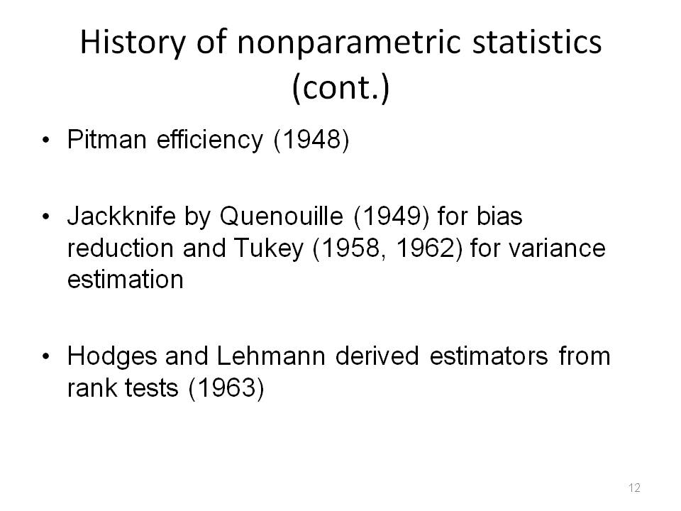
Also note the delete-a-group jackknife for variance estimation.

Many significant things in the nonparametric statistics world happened after this, of course, but this is a pretty good summary of the history without going into too much detail.
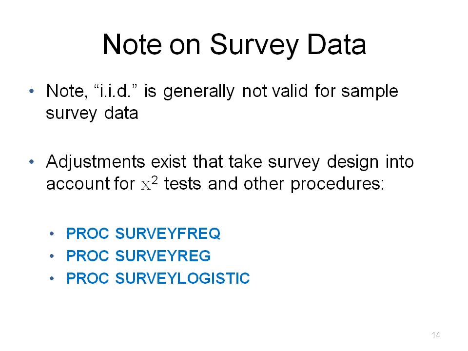
This needs to be said over and over when working with survey data.
This might not work with all weighting schemes however.
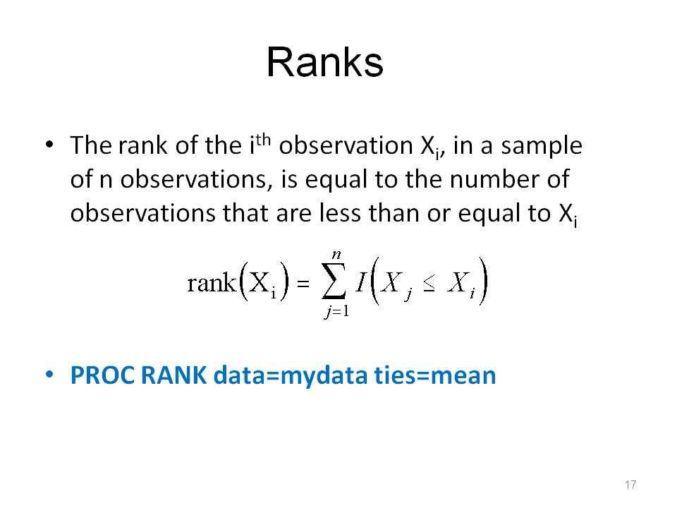
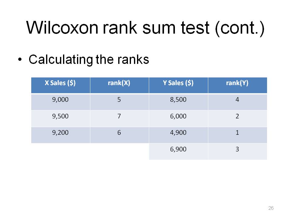
If you have your data, then the ranks, and say the X with the largest rank is now 100 times as big, the rank is the same, so there is built in resistance (i.e. performs well in the presence of outliers). Also, most data types can be transformed to ranks, so nonparametric statistics can handle interval, ratio, count data, ordinal, etc.
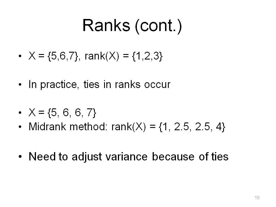
In theory, since distributions are assumed to be continuous, Prob(ties in ranks) = 0. In practice, ties occur all of the time (for example, due to issues of precision in measurement), so we need to make adjustments to ranks (there are several methods). Also one needs to make adjustments to standard errors in tests (because standard error would be incorrect).
In reality, there is no real "throwing away", because you still have kept the original data. You're just computing T(rank(X)) and using it for inference. A sensible question is, "How well are the variates (X) correlated with their ranks (rank(X))?" We'll look at a different, more sophisticated way to measure this idea of efficiency later on (Pitman).
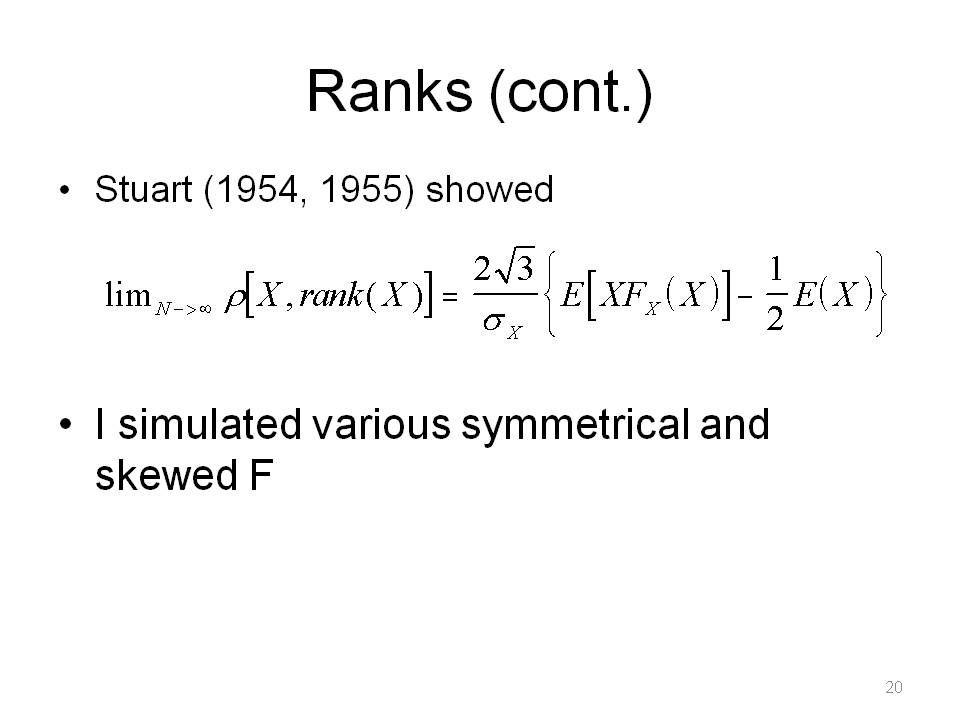
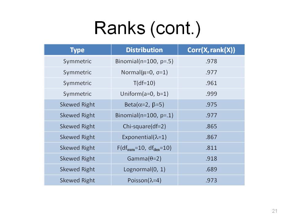
I simulated 1,000,000 draws of X and calculated rank(X), for each distribution. Note that these "skewed right" type of distributions are ones we often encounter in economic data. Remember, the point is we really never know what the true F is.
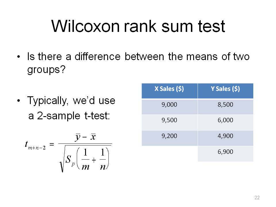
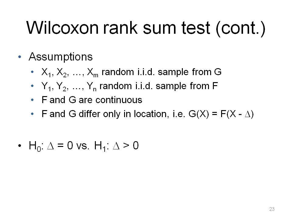
This is a so-called "distribution free" test statistic example. The data is random sample of m observations from a population with continuous probability distribution F, and an independent random sample of n observations from a second population with continuous probability distribution G. The null hypothesis asserts that the two random samples can be viewed as a single sample of size N = m + n from a common known population with unknown distribution F. The purpose is to detect differences in the distribution functions based on independent random samples from two populations.
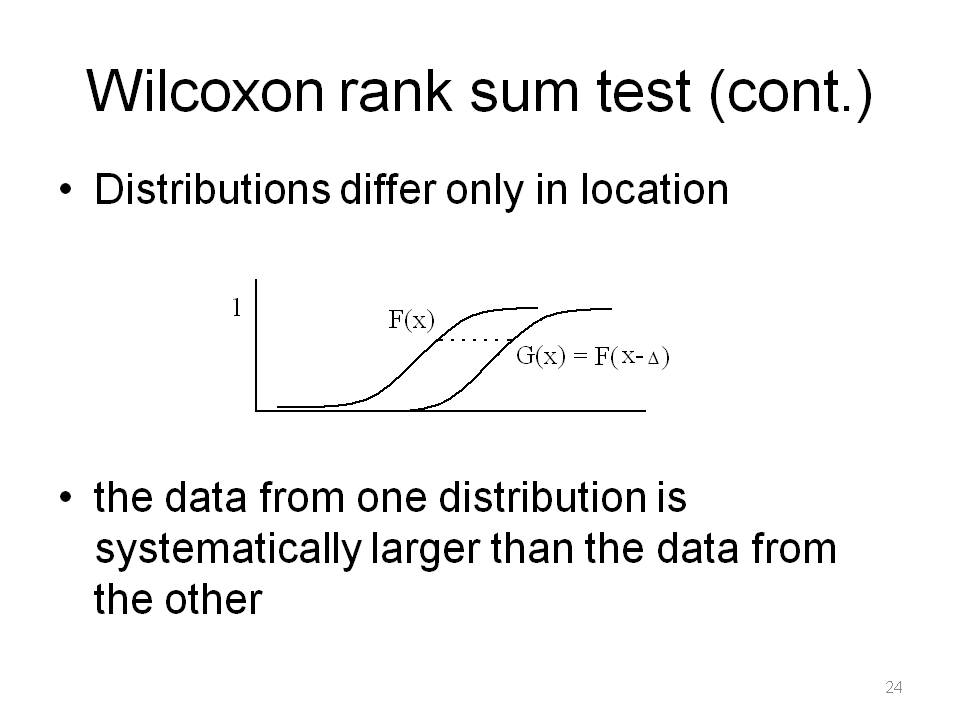
The logic is, if data from one distribution is systematically larger than the data from the other, then the ranks from that distribution are systematically larger than the ranks from the other.

Noe that the distribution of W does not depend on the distribution of X or Y, only m and n.
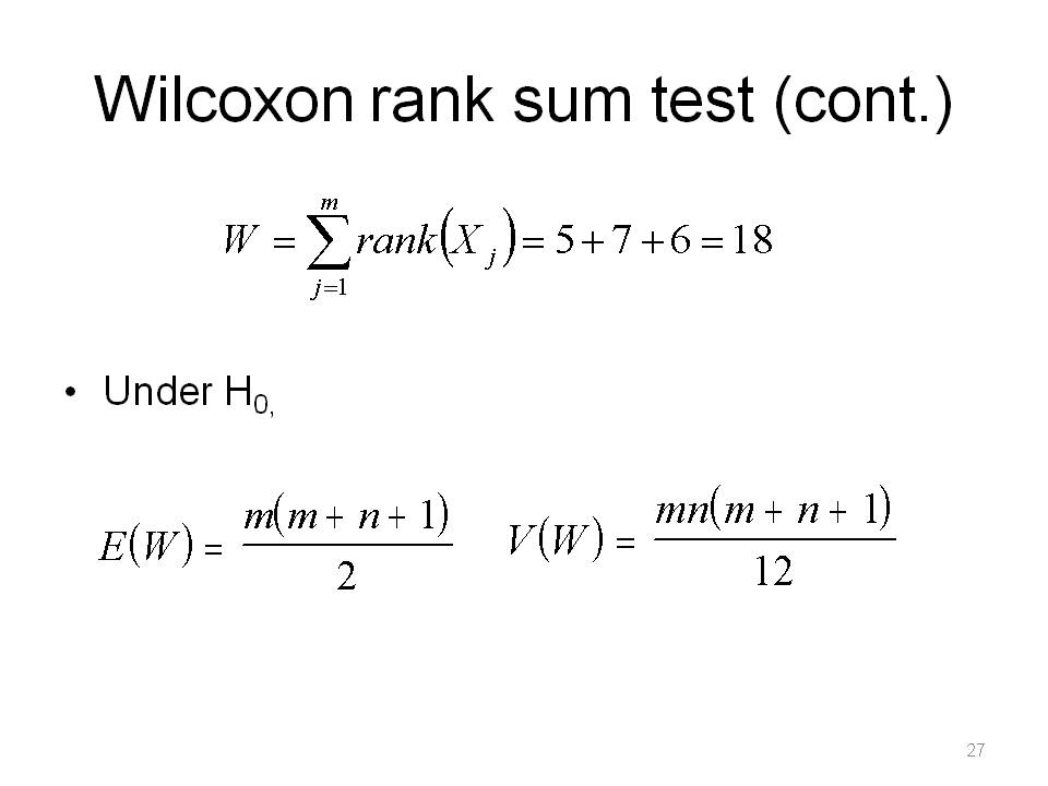
I won't derive E(W) and V(W). The derivation is on p. 116 of Nonparametric Statistical Methods, by Hollander and Wolfe. Note that E(W) = 12 for our example. Also note that there are no ties in ranks. If there are ties, V(W) would need to be adjusted.
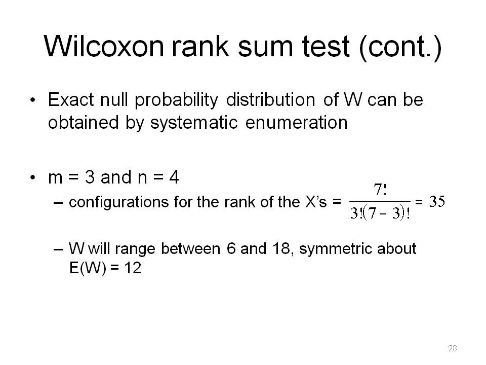
The smallest value of W: (1,2,3) = 6, and the largest value of W: (5,6,7) = 18.
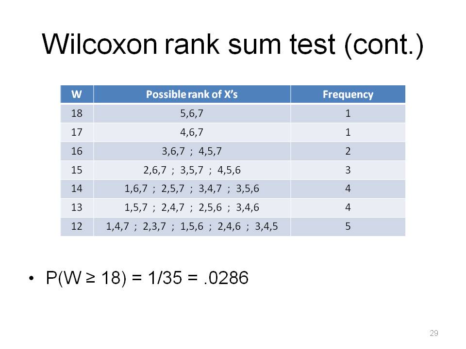
This is symmetric about 12 (so I won't fill in the whole table for W < 12). This listing of all possible combinations idea is why P-values are often said to be "exact" in many nonparametric statistics methods.
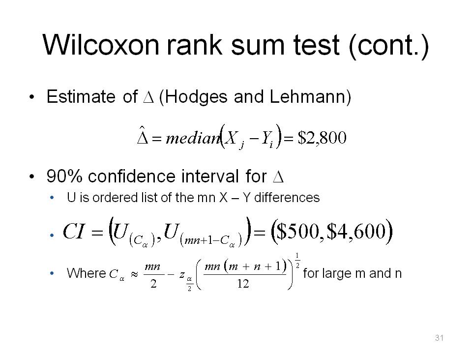
Calculate C_alpha, then the lower end point is the X-Y difference that occupies position C_alpha in the list of mn ordered X-Y differences. Note that the C_alpha has the form of a lower end point of a confidence interval using normal theory.
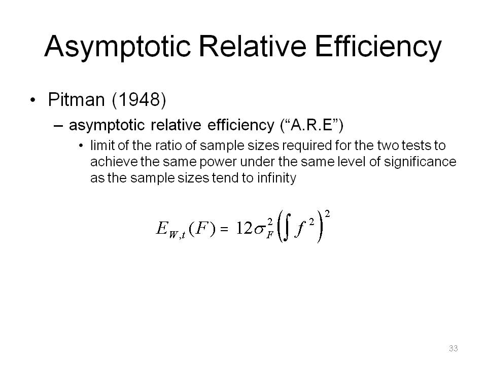
There are many variables are involved in testing: two tests, two hypotheses, sample sizes, alpha, power, the true underlying distribution(s), etc. Power is the probability of correctly rejecting H0, ie rejecting H0 when H1 is true, ie. P(reject H0 | H1 is true). W is Wilcoxon rank sum test, t is the normal theory two-sample t-test. One can calculate the asymptotic relative efficiency for other tests and distributions too, of course. This is independent of alpha and beta in the limit.
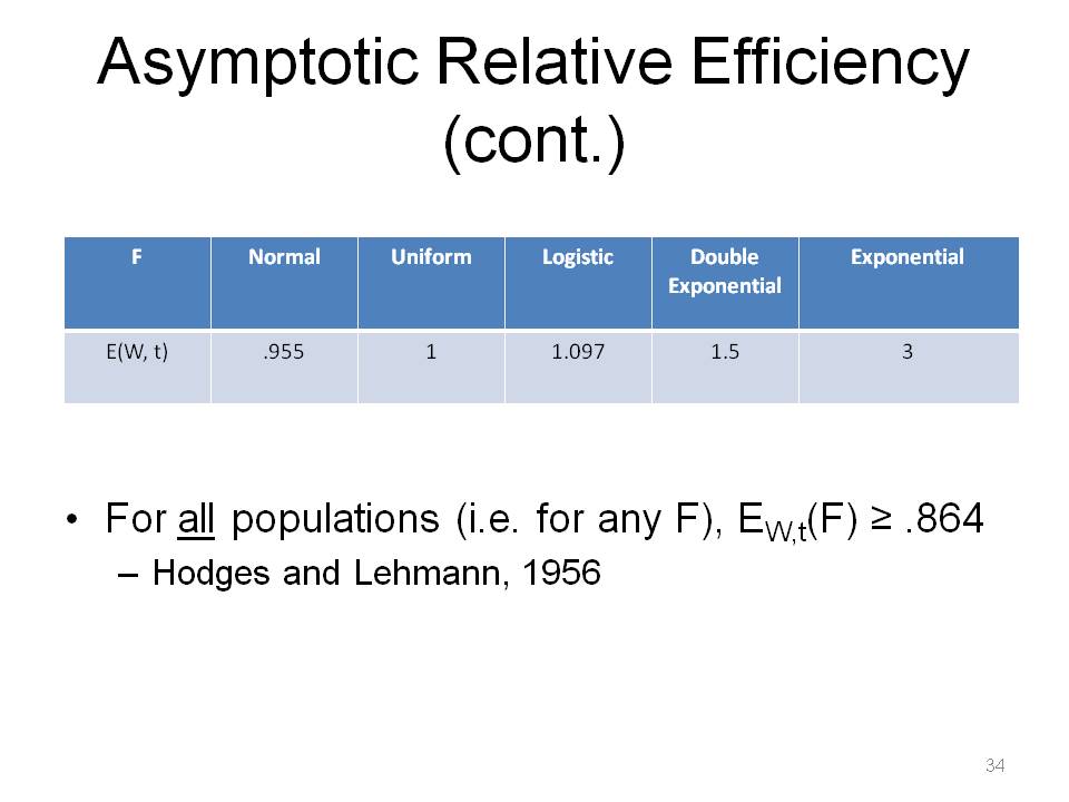
The interpretation is that the Wilcoxon test requires only 5% more observations to match the power of the two-sample t-test, when the distribution is Normal. When F is normal, ie the "home turf" of the t-test, the t-test is objectively more powerful, but you're not losing much by using the Wilcoxon, only about 5%. A Wilcoxon test using a sample size of n is as efficient as a two-sample t-test using a sample size of 3n when the distribution is Exponential. Notice E_W,t(F) >= .864 is a REMARKABLE result. The MOST efficiency one can lose when employing the Wilcoxon test instead of the two-sample t-test is about 14%. Again, remember we never know the true F.
Now I will shift gears and talk about various nonparametric methods used in survey work.
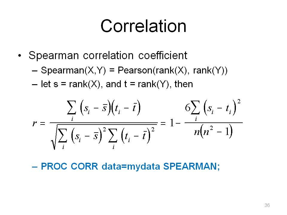
Measuring strength of relationship in statistics is important. We are familiar with Pearson correlation. It assumes linearity, tests based on r usually assume normality. The Spearman is somewhat difficult to interpret in a population parameter sense. Staff once asked me whether to report Corr(X,Y) and/or Corr(log(X),log(Y)) since they took a log transformation of X and Y. Report both, but can report Spearman(X,Y) = Spearman(log(X),log(Y)), because log is a monotonic function, so it doesn't change the ranking.
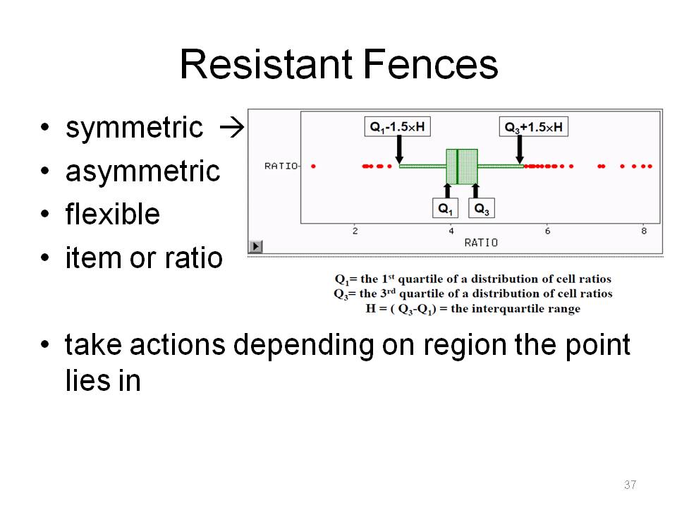
This is for outlier detection. Resistant fences also has a parametric justification, that if the data are normally distributed, we can compute the Type 1 error rate for an outlier. The k-values (1.5, 2, 3, etc.) are derived under normality assumptions.
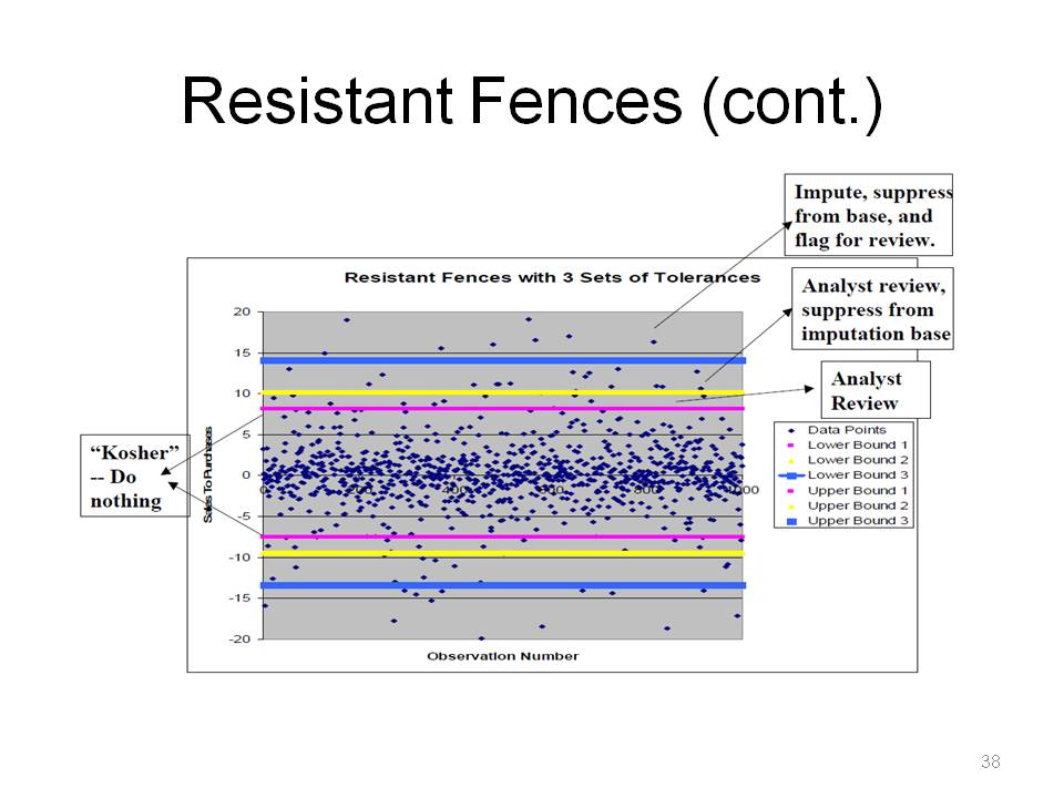
This is an example of regions: do nothing, flag for analyst review, impute, remove from imputation base.
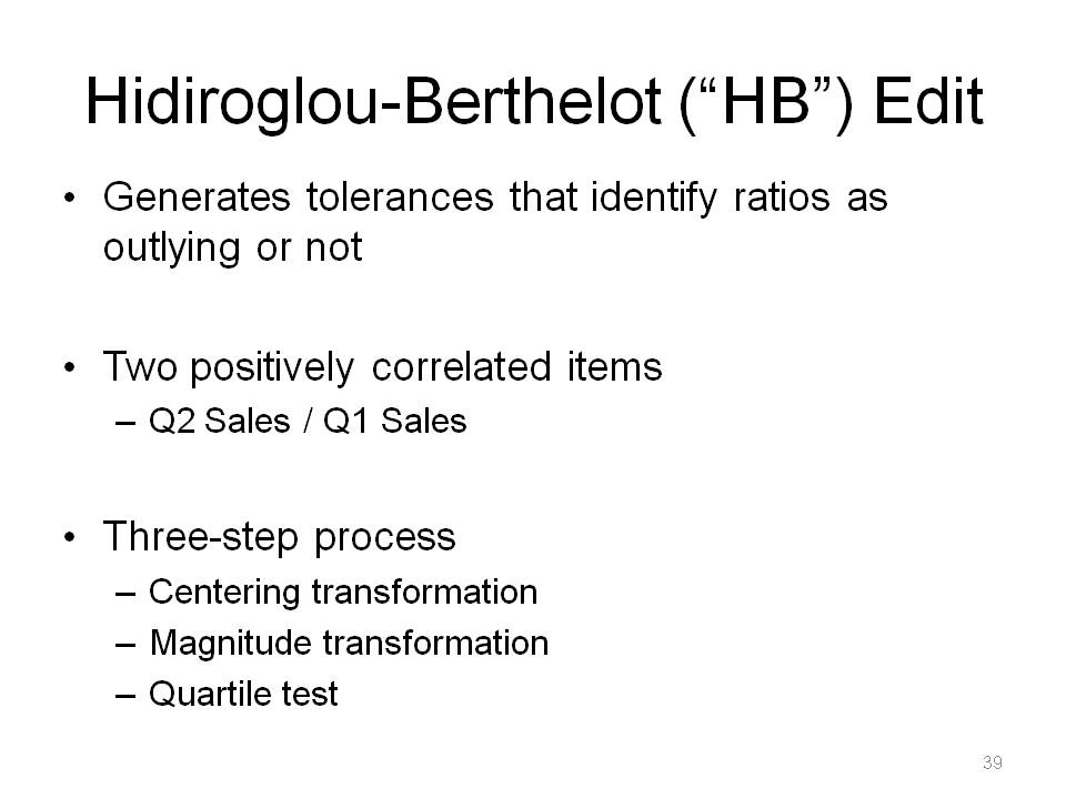
The data are centered, then transformed in such a way that they are expected to be fairly symmetric. The critical values are not derived assuming a parametric distribution for the transformed data. Don't use when you have negative or 0 values or uncorrelated or negatively correlated data.

Say R is ratio of current month to prior month for the ith unit. Half the S_i are less than 0, and half are greater than 0.
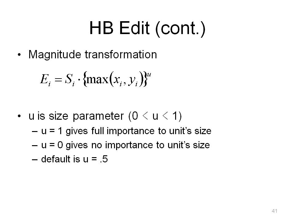
The size of the case is still disguised, so a second transformation is performed.
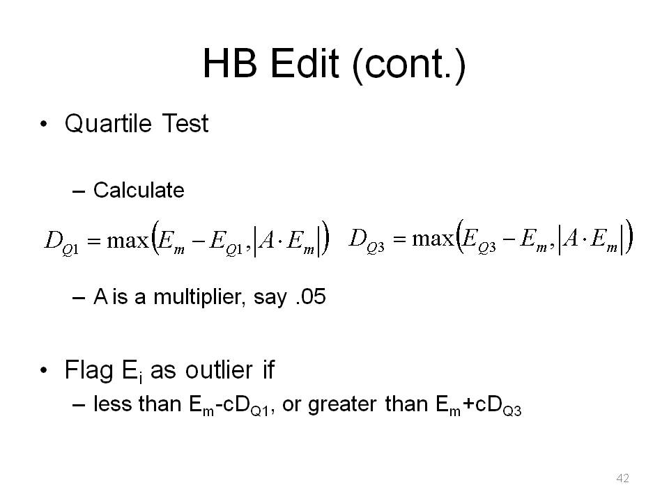
E_m is the median of the E_i's and E_Q1, is the first quartile of the E_i's, etc. The term A*E_m is used to protect against units clustered tightly about the median. Note, there is some subjectivity in setting parameters. You need feedback from analysts to determine good number of outliers vs workload middleground. The user determines values of c for regions, similar to Resistant Fences.
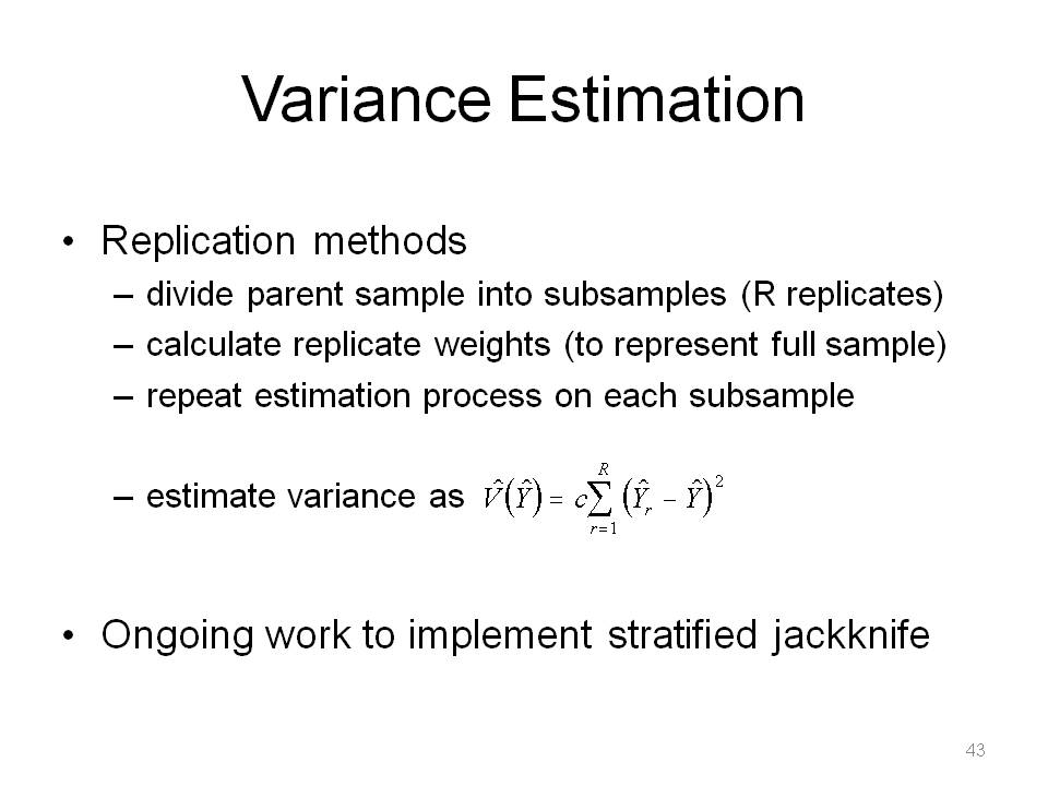
Replication side-steps the issue of obtaining formulas from theory for direct estimates. The design information is encoded into replicate weights. Replicate weights depend on replicate method. For Random Groups: G*WGT, i in g, 0 otherwise. For Delete-a-Group Jackknife, (G/G-1)*WGT, i not in g, 0 otherwise.
- c = 1/[R(R-1)] for random groups
- c = (R-1)/R for delete-a-group jackknife
- c = 1/R for balanced half sample
- c = 1/[(1-K)R] where 0 lt K lt 1 for modified half sample
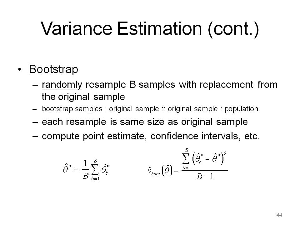
This is a na�ve bootstrap and modifications for complex survey settings exist. The bootstrap is like the jackknife, but it randomly does it. If without replacement, you'd just get the same set of numbers as the sample. If the sample is a good approximation of the population, the bootstrap method will provide a good approximation of the sampling distribution.
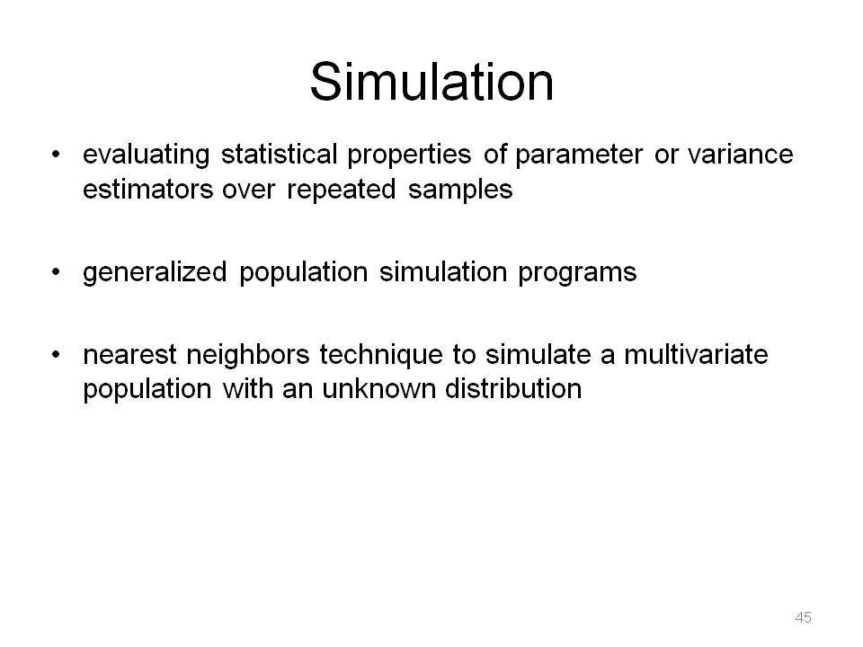
Simulation programs using multivariate lognormal distributions exist as well since we encounter skewed right distributions in economic survey work.
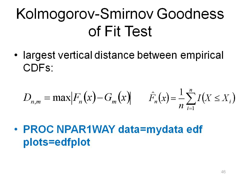
Note that 1 and 2 sample tests exist,
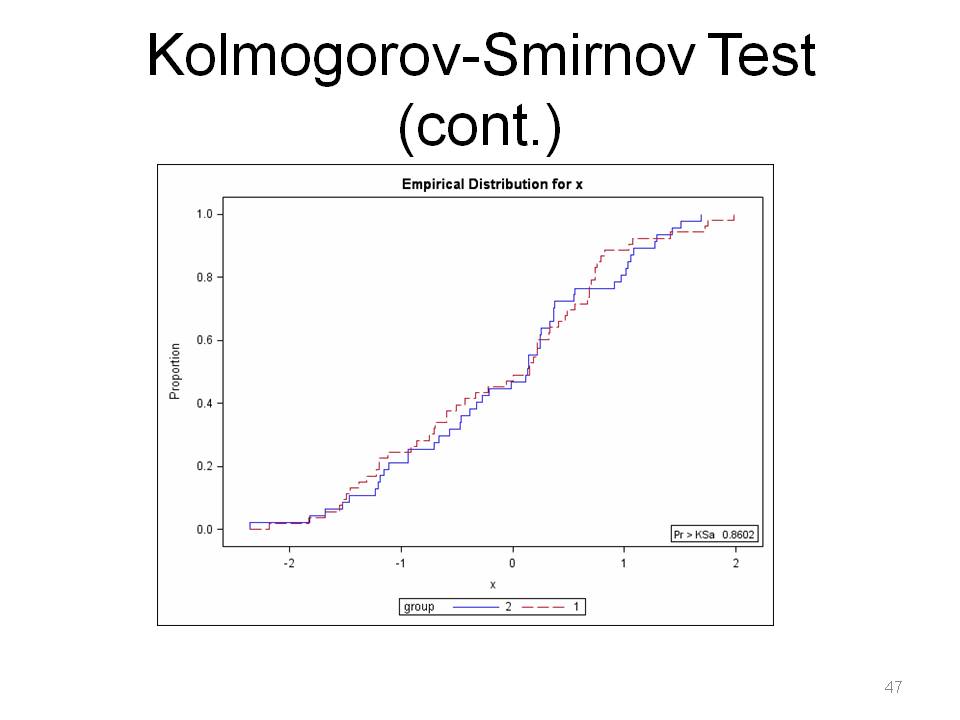
We fail to reject here, so F ~ G.
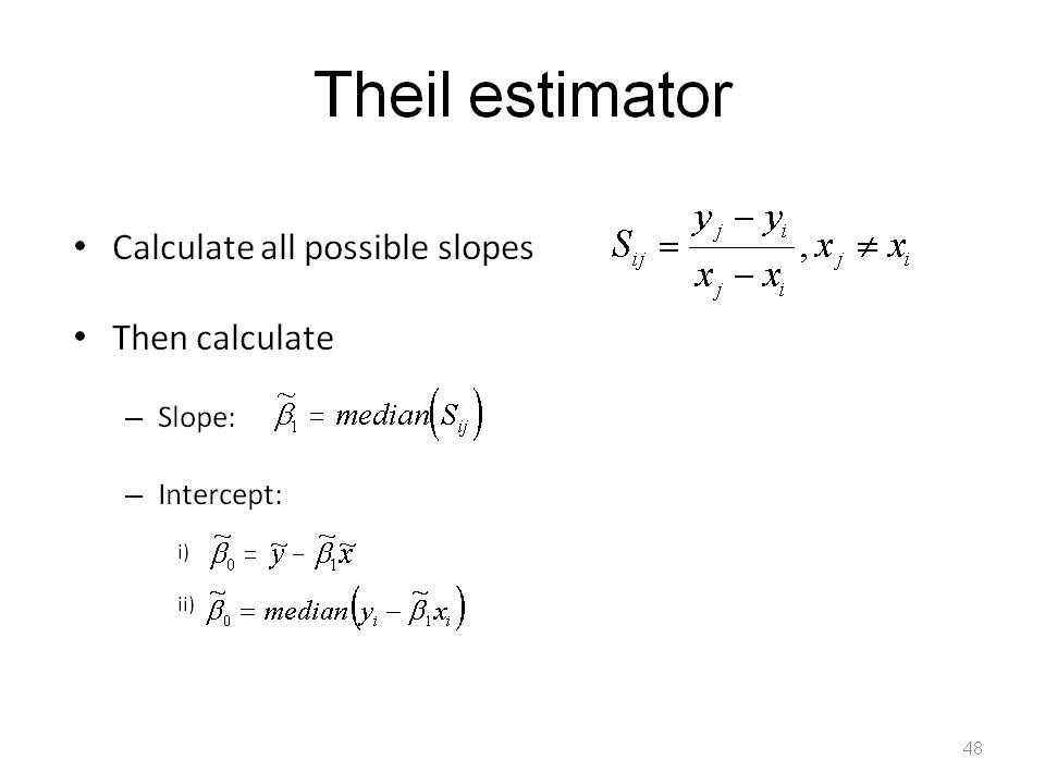
This still assumes familiar linear form, Yi = b0+b1Xi+ei, but residuals ~ continuous population with median 0. One needs to calculate the n(n-1)/2 individual sample slopes.

Note how outlier at x = 5 pulls least squares line upwards. This is less sensitive to gross errors than the classical least squares estimator, because it is the median of slopes, while the classical least squares estimator is a weighted average of slopes. The standard errors and CIs are obtained by bootstrapping, randomly sampling pairs of points with replacement and then using the percentile method for finding a confidence interval.
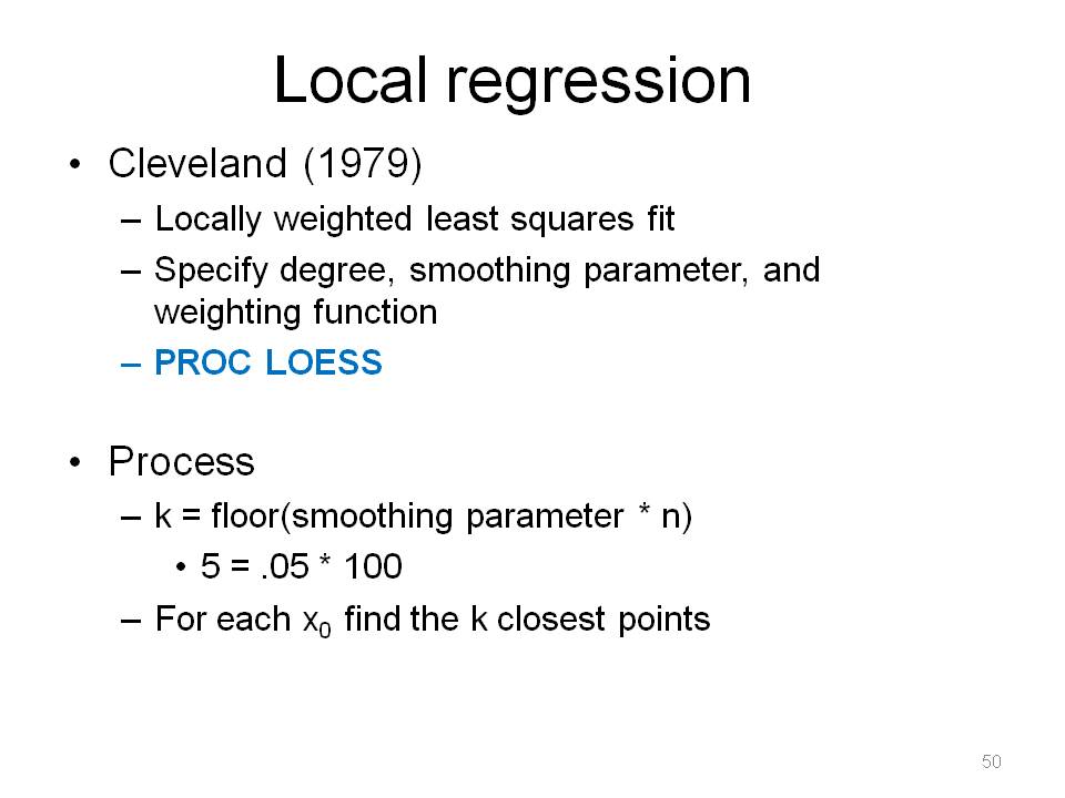
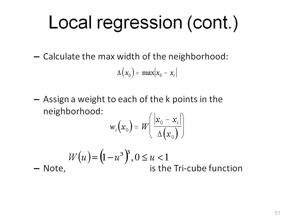
There is a long history on the subject of smoothing. LOESS uses the idea that things closer in space and time tend to be more similar than those further away.
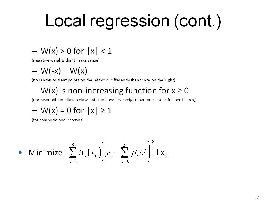
Note, because this uses least squares, it can be sensitive to outliers, however a robust method does exist (Cleveland).
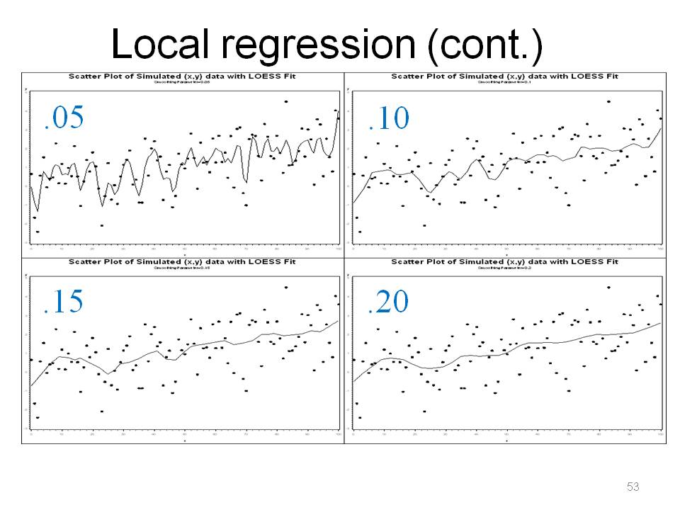
One can also get confidence intervals and interpolate. A smoothing parameter of .05, means going to use 5% of points around that point in the weighted estimate. A smoothing parameter of .05 is probably "overfit" / "too local", picks up too much variation, kind of silly. A large smoothing parameter gives results that approach standard linear regression because you're taking 100% of the data into account to compute the coefficients. Note that the value of smoothing parameter can be chosen by an AICC criterion. This strikes a balance between the residual sum of squares and the complexity of the fit. Basically pick the smoothing parameter as large as possible to minimize the variability in the smoothed points without distorting the pattern in the data. LOESS is really, really good for understanding story of data, especially in "dense" scatterplots.
The first bullet can be GOOD or BAD. If you have evidence or really good theory to support a distributional assumption, it is probably good to NOT ignore that information.
The jackknife and bootstrap are not 'cure alls' because it depends on the form of the estimator: totals, ratio, etc.
I expect growth of nonparametric methods in survey work because of the need with complex surveys and messy and skewed economic data.
I hope you found the presentation informative.
Please anonymously VOTE on the content you have just read:
Like:Dislike: